If you have to use your hands and spend hours doing things manually in Excel, you aren’t getting the most out of the program. Excel formulas are known for being able to process a lot of data quickly and without much help from the user. Indeed, Excel can do a lot more than you might think. It’s hard to ignore how great it is at making large data sets easier to manage. Furthermore, almost all of the tasks you do by hand can be made effortless with advanced excel functions.
Do you need to combine two spreadsheets that have the same data? Unquestionably, Excel has a formula for that. Should we put the two tables together? Excel uses the “&” symbol. Do you want an overall look at how your sheet is doing right now? Certainly, Microsoft Excel also has a keyboard shortcut for it.
Here, in this blog, we will discuss the top five time saving advanced excel formulas. As a result, by learning the formulas, you can easily get hold of your data.
Before we hop into the formulas, let’s briefly understand what advanced excel formulas are.
What are Advanced Excel Functions?
“Advanced Excel Functions” refers to the tools and features of Microsoft Excel that make it easier to do complex mathematical calculations, statistical analysis, and other tasks.
They go beyond simple math and include functions like VLOOKUP, SUMIF, INDEX-MATCH, and more. With these functions, you can automate tasks, pull out specific data, do conditional calculations, and use Excel to its fullest for advanced data analysis and making decisions. These functions can save you time, make your work easier, and turn you into an Excel expert.
Finally, let’s discover Excel functions which are really useful.
Advanced Excel Functions List
We’ve put together a list of 5 advanced Excel formulas that can make long, boring, manual tasks take only a few seconds to do. These are formulas that every professional should know so they can save valuable time or impress their boss at a crucial time.
Do you want to learn an advanced excel course for free? Well, worry not, we’ve got you covered!
Here’s our Advanced Excel Full Course 2023 video covering the top excel functions and formulas.
The best part?
IT IS FREE!
So, what are you waiting for? Click the link now and become an Excel Master.
Now, let’s learn about the top five functions here.
VlookUP Advanced Excel Functions
The VLOOKUP formula in Excel is a powerful function that lets you search for a value in the leftmost column of a table and get related information from a different column. Here is how it works:
Formula: VLOOKUP(lookup_value, table_array, col_index_num, [range_lookup])
- Lookup_value: The value you want to find in the table’s leftmost column.
- Table_array: The group of cells that make up the table with the data.
- Col_index_num: The number of the column in the table from which you want to get the data.
- Range_lookup: This is an optional parameter that lets you say if you want an exact match or a close match. Set it to TRUE or leave it out if you want a close match. Set it to FALSE if you want an exact match.
Example:
Let’s say you have a table with the names of students and their grades. You want to search for a student’s name to find out what grade they have.
Table:

To find Carol’s grade using VLOOKUP, you would use the following formula:
=VLOOKUP(“Carol”, A2:B4, 2, FALSE)
Explanation:
- The lookup_value is “Carol” because we want to find her grade.
- The table_array is A2:B4, which represents the range containing the names and grades.
- The col_index_num is 2 because we want to retrieve the grade from the second column.
- Since we want an exact match, we set range_lookup to FALSE.
The VLOOKUP formula will search for “Carol” in the leftmost column (column A) and return her corresponding grade (95) from the second column (column B).
Also Read:
Shortcut Keys for Excel – A Complete List
INDEX Advanced Excel Functions
The INDEX function in Excel is a flexible way to get information from a specific cell in a group of cells. How it works is as follows:
Formula: INDEX(array, row_num, [column_num])
- Array: The range of cells or arrays from which you want to get data.
- Row_num: The number of the row in the array whose data you want to get.
- Column_num: Parameter is optional. The number of the column in the array where you want to get the data. If left out, the formula returns the whole row that row_num points to.
Example:
For example, you have a table with the names of products and how much they sold. You want to find out how much a certain product sold for.
Table:
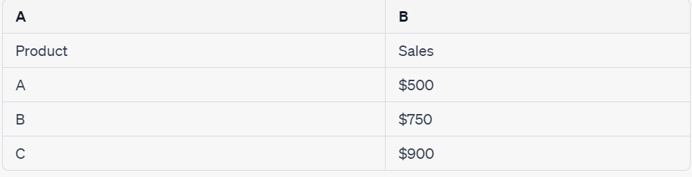
Here, to get the sales amount for product B using the INDEX formula, you would use the following formula:
=INDEX(B2:B4, 2)
Explanation:
- We chose B2:B4 for the array because we want to get data from the sales column.
- The row_num is 2 because we want to get the sales amount for product B, which is in the second row of the array.
- The value $750 will be returned by the INDEX formula, which is the amount of sales for product B in the table. If you add the optional column_num parameter, you can tell the function to get data from a specific column in the array.
Note: The INDEX formula is especially useful when combined with other functions like MATCH to make more advanced lookup and retrieval formulas in Excel.
MATCH Function in Excel
The MATCH function in Excel is a powerful way to find the location of a certain value in a range of cells. Here is how it works:
Formula: MATCH(lookup_value, lookup_array, [match_type])
- Lookup_value: The value in the lookup_array that you want to find.
- Lookup_array: The range of cells or array where you want to look for the lookup_value.
- Match_type: It is an optional parameter that tells the program what kind of match you want. Set it to 1 or leave it blank (the default) for a close match, set it to 0 for an exact match, and set it to -1 for a close match in descending order.
Example:
Let’s say you have a list of cities in column A and you want to use the MATCH formula to find out where a certain city is in the list.
Column A:

Now, with the MATCH formula, you would use the following formula to find where “Tokyo” is:
=MATCH(“Tokyo”, A1:A4, 0)
Explanation:
- We put “Tokyo” as the lookup_value because we want to find its location.
- The range where we want to look for “Tokyo” is A1:A4, which is what the lookup_array is.
- For an exact match, we set match_type to 0.
- The MATCH formula will search the lookup_array for “Tokyo” and give back the position of the first exact match. In this case, it will return the number 3 because “Tokyo” is in the third row of the lookup_array.
In any case, you can use the MATCH function along with other functions, such as INDEX, to get specific information about the position that was matched.
SUMIF Function
The SUMIF function in Excel is a powerful way to add up the values in a range based on a condition or set of criteria. How it works is as follows:
Formula: SUMIF(range, criteria, [sum_range])
- Range: The range of cells you want to use to see how well they meet the criteria.
- Criteria: The condition or set of rules that decides which cells to add up.
- Sum_range: Parameter is optional. The range of cells you’d like to add up. If you don’t include it, the formula will add up all the cells in the range parameter.
Example:
In this case, imagine you have a sales data table with product names in column A and sales amounts in column B. You want to figure out how much a certain product sold in total.

Certainly, to figure out the total sales for product A using the SUMIF formula, you would use the following formula:
=SUMIF(A2:A5, “A”, B2:B5)
Explanation:
- For example, we want to look at the names of the products, so the range is from A2 to A5.
- The criteria is “A” because we want to include cells where the name of the product is “A.”
- The sum_range is from B2 to B5 because we want to add up the sales for each product.
- The SUMIF formula will add up all the sales amounts in column B that meet the “A” criteria in column A. In this case, it will return $900, which is how much product A made in sales.
Moreover, you can use the SUMIF formula to do different kinds of calculations based on certain conditions. Without a doubt, this makes it easier to analyze and summarize your data.
IF AND FORMULA IN EXCEL
The IF AND function in Excel is a combination of the IF function and the AND function. It lets you test if two or more conditions are true. Here is how it works:
Formula: =IF(AND(condition1, condition2, ...), value_if_true, value_if_false)
- condition1, condition2,…: These are the logical conditions you want to check.
- Value_if_true: What to do or how much something is worth if all the conditions are met.
- Value_if_false: If any of the conditions aren’t met, the value or action to take.
Explanation:
For instance, you have a system for grading students and you want to see if a student passed a course based on how well they did on two exams. Both tests must be passed with a score of 60 or higher. Therefore, you want “Passed” to show up if the conditions are met and “Failed” to show up if they are not.
Student A:
Exam 1: 75
Exam 2: 80
To use the IF AND formula to see if Student A passed, you would use the following formula:
=IF(AND(B2 > 60 AND C2 > 60), “Passed”, “Failed”)
Explanation:
- The first condition, B2>=60, checks to see if Exam 1 score is at least 60.
- The second condition is C2>=60, which checks if the score on Exam 2 is at least 60.
- If both conditions are met (for example, if Student A gets at least 60 on both tests), the formula will show “Passed.”
- If any of the conditions are not true, such as if Student A gets less than 60 on either test, the formula will show “Failed.”
In this case, both conditions are met because Student A got 75 and 80 on Exam 1 and Exam 2, respectively. So, “Passed” will be shown by the formula.
Indeed, you can use the IF AND formula to do complex logical tests with multiple conditions. This lets you make decisions and take actions based on the conditions.
Conclusion
On the whole, we have discussed five advanced excel functions above. Of course, there are many more to the list. In fact, to learn about the top advanced excel formulas, do visit our youtube channel. To illustrate, we have covered the top excel formulas along with simple and easy to understand explanations. Microsoft Excel is almost a must-have in the modern workplace, but it doesn’t have to be hard to learn. Undeniably, if you can make it work for you, your output will go up dramatically.